Formulas 1: SUM, AVERAGE, COUNTIF, SUMIF
Four formulas answer "how much", "how much on average", "how many of these" and "how much for these".
Anatomy of a formula
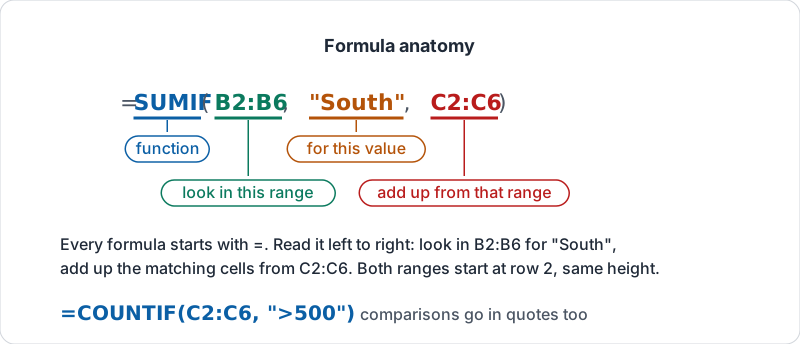
Every formula starts with an equals sign, then a function name, then its inputs in brackets separated by commas:
=SUM(C2:C40)
C2:C40 is a range: column C from row 2 to row 40. Start ranges at row 2 so the header is not included. If the table will grow, use the whole column (C2:C) and the formula keeps up.
Put formulas in a separate area (a summary block to the right, or a Summary sheet), never inside the data rows.
The parts of a SUMIF, labelled.
The four
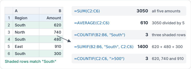
Use this sample table for the examples. Region is column B, Amount is column C, rows 2 to 6.
| Row | B Region | C Amount |
|---|---|---|
| 2 | South | 620 |
| 3 | North | 740 |
| 4 | South | 480 |
| 5 | East | 910 |
| 6 | South | 300 |
| Question | Formula | Result |
|---|---|---|
| Total of all amounts | =SUM(C2:C6) |
3050 |
| Average amount | =AVERAGE(C2:C6) |
610 |
| How many South rows | =COUNTIF(B2:B6, "South") |
3 |
| Total amount for South | =SUMIF(B2:B6, "South", C2:C6) |
1400 |
| How many amounts over 500 | =COUNTIF(C2:C6, ">500") |
3 |
Read SUMIF left to right: look in this range for this value, and add up the matching cells from that range. The two ranges must be the same height.
The same five rows with each answer worked out.
Criteria rules
- Text criteria go in double quotes:
"South". Matching ignores capital letters, so “south” also counts (another reason to use dropdowns). - Comparisons go in quotes too:
">500","<=100","<>Cancelled"(not equal). - A criterion can point at a cell:
=SUMIF(B2:B, F1, C2:C)totals whatever region is typed in F1. Change F1, the total changes. - To match the start of a word use a wildcard:
"Store*"matches Store A and Store B. - Two conditions at once? Use the plural forms:
=COUNTIFS(B2:B, "Paid", C2:C, ">500")counts rows that are Paid and over 500;SUMIFSworks the same way with the sum range first.
When the answer looks wrong
| Symptom | Likely cause |
|---|---|
| Total is too low | Some amounts are text (sit on the left of the cell) |
| COUNTIF returns 0 | A trailing space in the data or the criterion, or a spelling variant |
| Average is too high | A total row is inside the range |
| Result is a date | The cell is formatted as a date; change the number format |
Try it now
In a sheet with a category column and an amount column, add a summary block to the right with four formulas: the overall total, the average, a COUNTIF for one category and a SUMIF for the same category. Check the SUMIF by filtering to that category and reading the total at the bottom of the screen.
Remember: SUM for how much, AVERAGE for typical, COUNTIF for how many match, SUMIF for how much for the ones that match. Criteria go in quotes.
Checking your progress…